Domain-Dependent Policy Learning using Neural Networks for Classical Planning (2/4)

This post as the second of the series about my undergraduate thesis will cover the underlying architecture of Action Schema Networks.

Action Schema Networks

Action Schema Networks, short ASNets, is a neural networks architecture proposed by Sam Toyer et al. [1, 2] for application in automated planning. The networks are capable of learning domain-specific policies to exploit on arbitrary problems of a given (P)PDDL domain. This post will cover the general architecture and design of the networks as well as their training and exploitation of learned knowledge will be explained. Lastly, Sam Toyer’s empirical evaluation of ASNets on planning tasks will be presented.

Architecture

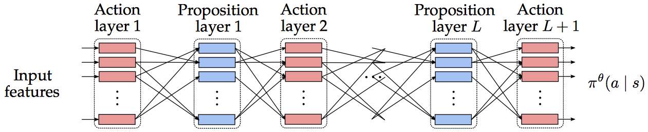
ASNets are composed of alternating action and proposition layers, containing action and proposition modules for each ground action or proposition respectively, starting and ending with an action layer. Overall the network computes a policy $\pi^\theta$, outputting a probability $\pi^\theta(a \mid s)$ to choose action $a$ in a given state $s$ for every action $a \in \mathcal{A}$. One naive approach to exploit this policy during search on planning tasks would be to greedily follow $\pi^\theta$, i.e. choosing $argmax_{a} \pi^\theta(a \mid s)$ in state $s$.

The following figure out of Toyer’s thesis [1] illustrates an ASNet with $L$ layers.

Action modules

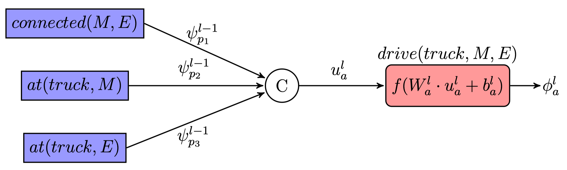
Each action module in an action layer $l$ represents a ground action $a$ and computes a hidden representation

$$\phi^l_a = f(W^l_a \cdot u^l_a + b^l_a)$$

where $u^l_a \in \mathbb{R}^{d^l_a}$ is an input vector, $W^l_a \in \mathbb{R}^{d_h \times d^l_a}$ is a learned weight matrix and $b^l_a \in \mathbb{R}^{d_h}$ is the corresponding bias. $f$ is a nonlinear function, e.g. RELU or tanh, and $d_h$ represents a chosen hidden representation size. The input is constructed as follows

$$u^l_a = \begin{bmatrix} \psi^{l-1}_1 \ \cdots \ \psi^{l-1}_M \end{bmatrix}^T$$

where $\psi^{l-1}_i$ is the hidden representation of the proposition module of the $i$-th proposition $p_i$ related to $a$ in the preceding proposition layer. Proposition $p \in \mathcal{P}$ is said to be related to action $a \in \mathcal{A}$ iff $p$ appears either in the precondition $pre_a$, add- $add_a$ or delete-list $del_a$ of action $a$. This concept of relatedness is essential for the sparse connectivity of ASNets essential for their weight sharing and efficient learning.

Coming back to the dummy planning task introduced in the previous post, where a package has to be delivered from Manchester to Edinburgh, the action module for $drive(truck, M, E)$ would look like this:

Note that the number of related propositions $N$ of two actions $a_1$ and $a_2$, which are instantiated from the same action schema of the underlying domain, will always be the same. Hence, each action module of e.g. $drive$ actions will have the same structure based on the action schema and relatedness. This is used in ASNets to share weights matrices $W^l_a$ and bias $b^l_a$ among all actions of the same action schema as $a$ in layer $l$. Through this approach, ASnets are able to share these parameters among arbitary instantiated problems of the same domain as these all share the same action schemas.

Action modules of the very first action layer receive specific input vectors $u^1_a$ containing binary features representing the truth values of related propositions in input state $s$, values indicating the relevance of related propositions for the problem’s goal as well as a value showing whether $a$ is applicable in $s$. Additionally, Sam Toyer et al. experimented with heuristic features regarding disjunctive action landmarks, computed for the LM-cut heuristic [3], as additional input to overcome limitations in the receptive field of ASNets. Otherwise, ASNets are only able to reason about action chains with length at most $L$.

For the output action layer respectively, the network has to output a policy represented by a probability distribution $\pi^\theta(a \mid s)$. This is achieved using a masked softmax activation function, where a mask $m$ is applied to ensure that $\pi^\theta(a \mid s) = 0$ iff $pre_a \nsubseteq s$, i.e. only applicable actions receive nonzero probability. The mask represents this as binary features with $m_i = 1$ iff $pre_{a_i} \subset s$ and $m_i = 0$ otherwise. Overall, the activation function computes the probability $\pi_i = \pi^\theta(a_i \mid s)$ as follows for all actions $\mathcal{A} = {a_1, …, a_N}$: $$\pi_i = \frac{m_i \cdot \exp(\phi^{L + 1}_{a_i})}{\sum_{j=1}^N m_j \cdot \exp(\phi^{L + 1}_{a_j})}$$

Proposition modules

Proposition modules are constructed very similarly to action modules but only occur in intermediate layers. Therefore a hidden representation produced by the module for proposition $p \in \mathcal{P}$ in the $l$-th layer looks like the following $$\psi^l_p = f(W^l_p \cdot v^l_p + b^l_p)$$ where $v_p^l \in \mathbb{R}^{d_p}$ is an input vector and $W^l_p$, $b^l_p$ represent the respective weight matrix and bias vector and $f$ is the same nonlinearity applied in action modules. The main difference between proposition and action modules is that the number of actions related to one proposition can vary making the input construction slightly more complicated.

To deal with this variation and be able to share weights among proposition modules as for action modules, the input feature vector’s dimensionality $d_p^l$ has to be equal for all propositions with the same underlying predicate. Therefore the action schemas $A_1, …, A_S$ referencing the predicate of proposition $p$ in their preconditions, add or delete list are collected. When building the hidden representation of proposition p, all related grounded actions from the listed action schemas are considered with action module representations of the same action schema being combined to a single $d_h$-dimensional vector using a pooling function:

$$v^l_p = \begin{bmatrix} pool({\phi^l_a \mid op(a) = A_1 \wedge R(a, p)}) \ \cdots \ pool({\phi^l_a \mid op(a) = A_S \wedge R(a, p)}) \end{bmatrix}^T$$

$op(a)$ reflects the action schema of grounded action $a$ and $R(a, p)$ denotes if $a$ and $p$ are related.

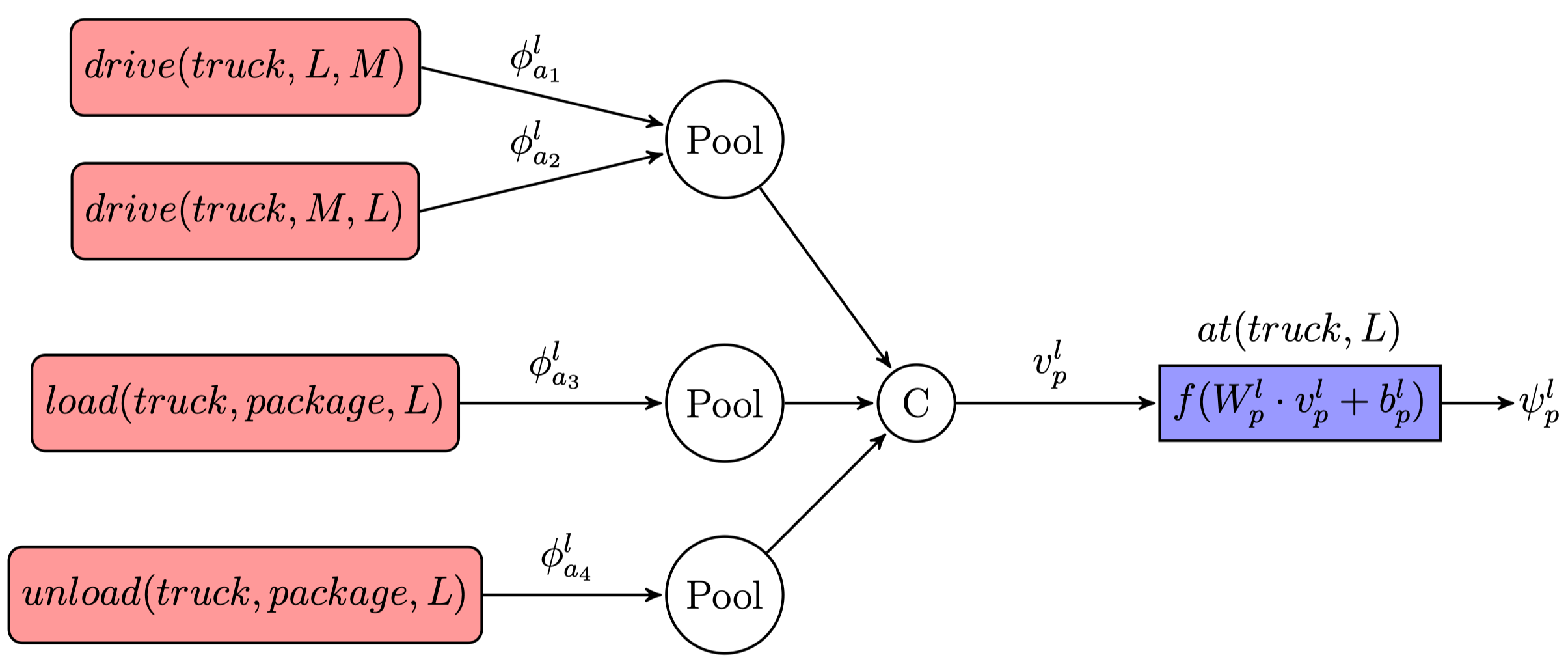
The figure illustrates a proposition module for $at(truck, L)$ in the described planning task of the previous post.

Supervised Training

During training, the ASNet is executed on small problems from a domain to learn weights, which still lead to an efficient policy on larger problems of the same domain. The proposed supervised training algorithm, proposed by Sam Toyer et al., relies on a teacher policy.

At the beginning of the training, weights and bias are initialized by employing the Glorot initialisation, or Xavier initialisation [4], using a zero-centred Gaussian distribution. After initializing the parameters, the network is exploring the state space of each training problem during multiple epochs. Starting from the problem’s initial state $s_0$, the exploration follows the network policy $\pi^\theta$ and stops when a limited amount of states have been traversed, a goal or dead-end state have been reached. Dead-ends can be detected efficiently using a delete-relaxed heuristic [5]. Let the set of explored states in epoch $e$ be denoted as $S_{exp}^e$.

Additionally, for every $s \in S_{exp}^e$ a teacher policy (usually an optimal policy) $\pi^∗$ is used to extract all states encountered when following the policy from $s$. All these states are collected in the set $S_{opt}^e$ to ensure that the network is always trained with ``good” states, while $S_{exp}^e$ is essential to allow the network to improve upon its performance in already visited states. Afterwards, the set of training states $\mathcal{M}$ is updated as $\mathcal{M} = \mathcal{M} \cup S_{exp}^e \cup S_{opt}^e$. After each exploration phase the ASNet’s weights $\theta$ are updated using the loss function $$\mathcal{L}_\theta(\mathcal{M}) = \frac{1}{|\mathcal{M}|} \sum_{s \in \mathcal{M}} \sum_{a \in \mathcal{A}} \pi^\theta(a \mid s) \cdot Q^*(s, a)$$ where $Q^*(s,a)$ denotes the expected cost of reaching a goal from $s$ by following the policy $\pi^*$ after taking action a. The parameter updates are performed using minibatch *stochastic gradient descent* to save the significant expense of computing gradients on the entire state collection $\mathcal{M}$ and can generally converge faster [6]. The Adam optimization algorithm, proposed by Kingma and Ba [7], is used to optimise $\theta$ in a direction minimizing $L_\theta(\mathcal{M})$.

Exploration is stopped early whenever an early stopping condition is fulfilled, where the network policy $\pi^\theta$ reaches a goal state in at least $99.9%$ of the states in $\mathcal{M}$ during the last epoch and the success rate of $\pi^\theta$ did not increase by more than $0.01%$ over the previous best rate for at least five epochs.

Empirical Evaluation

Sam Toyer conducted an experiment comparing ASNets to state-of-the-art probabilistic planners LRTDP [8], ILAO$^*$ [9] and SSiPP [10] to be able to evaluate their performance. All experiments were run with the admissible LM-cut and inadmissible $h^{add}$ heuristic and were limited to 9000s and 10Gb memory.

The ASNet was trained using two layers, a hidden representation size $d_h = 16$ for each module and the ELU activation function [11] for each domain using small problem instances. The learning rate during training was 0.0005 and a batch size of 128 was utilized for the Adam optimization. Additionally, $L_2$ regularization with $\lambda = 0.001$ on the weights and dropout [12] with $p = 0.25$ on the outputs of all intermediate layers was used to prevent overfitting. Training was limited at two hours. As the teacher policy in the ASNets LRTDP with $h^{LM−cut}$ and $h^{add}$ was employed.

Three probabilistic planning domains were used in the evaluation: CosaNostra Pizza [13], Probabilistic Blocks World [14] and Triangle Tire World [15]. Besides probabilistic planning, Sam Toyer also briefly evaluated ASNets on the deterministic classical planning domain Gripper [16] against Greedy best-first search (GBFS), $A^*$ using the $h^{LM-cut}$ and $h^{add}$ heuristics, LAMA-2011 [17] and LAMA-first, which won the International Planning Competition (IPC) 2011.

ASNets performed comparably better on large problems where the required training truly pays off. They were able to significantly outperform all baseline planners on large problem instances of the CosaNostra Pizza and Triangle Tire World domains learning optimal or near optimal policy for many problems. For the Probabilistic Blocks World domain, the LM-cut policy was too expensive to compute and the exploration using the $h^{add}$ teacher policy was insufficient to outperform the baseline planners for complex tasks.

In deterministic planning, ASNets took significantly more time to train and evaluate compared to most baseline planners. The solutions of ASNets using additional heuristic input features were found to be optimal on all problems, but without such input the networks were unable to solve even problems of medium size. However, the LAMA planners outperformed ASNets in the considered problems finding optimal solutions significantly faster. It should be noted that the experiment primarily focused on probabilistic planning and the classical planning part was merely to show the ability of ASNets to be executed on these tasks. To measure and evaluate the performance of ASNets in classical deterministic planning, a comprehensive experiment would still be needed.

In the third post, I will explain my contributions to extending the capabilities of ASNets in deterministic automated planning and how these networks were integrated into the Fast-Downward planning system [18].

References

1. Toyer, S. (2017). Generalised Policies for Probabilistic Planning with Deep Learning (Research and Development, Honours thesis). Research School of Computer Science, Australian National University.
2. Toyer, S., Trevizan, F. W., Thiébaux, S., & Xie, L. (2017). Action Schema Networks: Generalised Policies with Deep Learning. CoRR, abs/1709.04271. Retrieved from http://arxiv.org/abs/1709.04271
3. Helmert, M., & Domshlak, C. (2009). Landmarks, Critical Paths and Abstractions: What’s the Difference Anyway? (pp. 162–169).
4. Glorot, X., & Bengio, Y. (2010). Understanding the difficulty of training deep feedforward neural networks. In Y. W. Teh & M. Titterington (Eds.), Proceedings of the Thirteenth International Conference on Artificial Intelligence and Statistics (Vol. 9, pp. 249–256). Chia Laguna Resort, Sardinia, Italy: PMLR. Retrieved from http://proceedings.mlr.press/v9/glorot10a.html
5. Hoffmann, J., & Nebel, B. (2001). The FF Planning System: Fast Plan Generation Through Heuristic Search. Jair, 14, 253–302.
6. Li, M., Zhang, T., Chen, Y., & Smola, A. J. (2014). Efficient Mini-batch Training for Stochastic Optimization. In Proceedings of the 20th ACM SIGKDD International Conference on Knowledge Discovery and Data Mining (pp. 661–670). New York, NY, USA: ACM. https://doi.org/10.1145/2623330.2623612
7. Kingma, D., & Ba, J. (2014). Adam: A Method for Stochastic Optimization. International Conference on Learning Representations.
8. Bonet, B., & Geffner, H. Labeled RTDP: Improving the Convergence of Real-Time Dynamic Programming (pp. 12–21).
9. Hansen, E. A., & Zilberstein, S. (2001). LAO: A heuristic search algorithm that finds solutions with loops. Artificial Intelligence, 129, 35–62.
10. Trevizan, F., & Veloso, M. M. (2014). Short-sighted stochastic shortest path problems. Artificial Intelligence, 216.
11. Clevert, D.-A., Unterthiner, T., & Hochreiter, S. (2015). Fast and Accurate Deep Network Learning by Exponential Linear Units (ELUs). CoRR, abs/1511.07289. Retrieved from http://arxiv.org/abs/1511.07289
12. Srivastava, N., Hinton, G., Krizhevsky, A., Sutskever, I., & Salakhutdinov, R. (2014). Dropout: A Simple Way to Prevent Neural Networks from Overfitting. Journal of Machine Learning Research, 15, 1929–1958. Retrieved from http://jmlr.org/papers/v15/srivastava14a.html
13. Stephenson, N. (1992). Snow Crash. Bantam Books.
14. Younes, H. L. S., Littman, M. L., Weissman, D., & Asmuth, J. (2005). The First Probabilistic Track of the International Planning Competition. Jair, 24, 851–887.
15. Little, I., & Thiebaux, S. (2007). Probabilistic Planning vs Replanning. In ICAPS Workshop on the International Planning Competition: Past, Present and Future.
16. Long, D., Kautz, H., Selman, B., Bonet, B., Geffner, H., Koehler, J., … Fox, M. (2000). The AIPS-98 Planning Competition. Aim, 21(2), 13–33.
17. Richter, S., Westphal, M., & Helmert, M. (2011). LAMA 2008 and 2011 (planner abstract). In IPC 2011 planner abstracts (pp. 50–54).
18. Helmert, M. (2006). The Fast Downward Planning System. J. Artif. Int. Res., 26(1), 191–246. Retrieved from http://dl.acm.org/citation.cfm?id=1622559.1622565